개요
이번 포스팅에는 R에서 함수를 정의/호출하는 방법을 알아본다.
코드중심의 설명이기 때문에 본문 보다는 코드의 주석이 집중적으로 추가되어 있으니 참고 바란다.
함수 정의
피타고라스의 정리를 한번 구현해보자.
> hypotenuse <- function(x, y) {
+ sqrt(x^2+y^2)
+ }

> hypotenuse <- function(x, y) sqrt(x^2+y^2) # inline으로 나타낼 수 있음

> hypotenuse(3, 4)
[1] 5

> hypotenuse(x=3, y=4) # same as hypotenuse(y=4, x=3)
[1] 5
함수 argument 정보 보기
> hypotenuse <- function(x=5, y=12) sqrt(x^2+y^2)

> args(hypotenuse)
function (x = 5, y = 12)
NULL

> formalArgs(hypotenuse)
[1] "x" "y"
함수 scope와 Global scope
> h <- function(x) {
+ k <- 2
+ k*(x+y)
+ }

> k
Error: object 'k' not found

> h(9)
Error in h(9) : object 'y' not found

> y <- 16

> h(9)
[1] 50
예제를 한번 더 보자면 아래와 같다.
> f <- function(x) {
+ a*x
+ }

> f(3)
Error in f(3) : object 'a' not found

> a <- 10

> f(3)
[1] 30

> g <- function(y) {
+ a <- 100
+ f(y)
+ }

> g(3)
[1] 30
함수 scope
위에서 정의한 f함수는 다른 함수에서 사용 할 수 있다. 시험문제로 내기 좋은 패턴이다.
예제를 하나 더 보도록 하자.
여담이지만 runif는 발음을 “run-if”가 아니라 “r-uniform”으로 발음한다. R을 쪼끔 아는지 모르는지 이걸로 테스트해보면 재밌을듯 하다.(농담)
> y <- 16

> h2 <- function(x) {
+ if(runif(1) > 0.5) y <- 12 # runinf(1)은 0~1사이의 랜덤값을 획득함
+ x*y
+ }

> replicate(10, h2(9)) # h2(9)를 10번 실행한다는 의미이다. 랜덤값에 따라 y는 16 아니면 12 둘중의 하나가 된다.
[1] 144 108 108 108 144 108 108 144 108 144
퀴즈
정답은 36이다.
벡터와 함수
아래와 같이 벡터를 입력값으로 받아 함수 계산을 할 수 있다. 시험문제로 내기 좋은 특징이다.
> normalize <- function(x) {
+ m <- mean(x)
+ s <- sd(x)
+ (x-m)/s
+ }

> x <- c(1, 3, 6, 10, 15)

> z <- normalize(x)

> mean(z) # almost 0
[1] -5.572799e-18

> sd(z)
[1] 1
하나 유의할 점은 normalize는 NA값이 하나라도 섞이면 모든 값이 NA로 바뀌므로 아래와 같은 처리가 필요하다.
> normalize(c(1, 3, 6, 10, NA))
[1] NA NA NA NA NA

> normalize <- function(x, na_remove=FALSE) {
+ m <- mean(x, na.rm=na_remove)
+ s <- sd(x, na.rm=na_remove)
+ (x-m)/s
+ }

> normalize(c(1, 3, 6, 10, NA), na_remove=TRUE)
[1] -1.0215078 -0.5107539 0.2553770 1.2768848

> normalize <- function(x, ...) {
+ m <- mean(x, ...)
+ s <- sd(x, ...)
+ (x-m)/s
+ }

> normalize(c(1, 3, 6, 10, NA), na.rm=TRUE)
[1] -1.0215078 -0.5107539 0.2553770 1.2768848 NA
함수작성 예제1
mysummary <- function(x, npar=TRUE, print=TRUE) {

  if (!npar) {
    center <- mean(x); spread <- sd(x)
    } else {
      center <- median(x); spread <- mad(x)
      }
  if (print & !npar) {
    cat(" Mean=", center, "\n", "SD=", spread, "\n")
    } else if (print & npar) {
      cat(" Median=", center, "\n", "MAD=", spread, "\n")
      }
  result <- list(center=center, spread=spread)
  return(result)
  }

  > mysummary(3) # 아래와 같이 리스트로 반환해준다.
   Median= 3
   MAD= 0
  $center
  [1] 3

  $spread
  [1] 0

  > # invoking the function
  > set.seed(1234)
  > x <- rpois(500, 4)
  > y <- mysummary(x)
  Median= 4
  MAD= 1.4826

  > # y$center is the median (4)
  > # y$spread is the median absolute deviation (1.4826)
  > y <- mysummary(x, npar=FALSE, print=FALSE)
  > y
  $center
  [1] 4.052
  $spread
  [1] 2.01927
  > # no output
  > # y$center is the mean (4.052)
  > # y$spread is the standard deviation (2.01927)
재귀함수, factorial
1 * 2 * 3 * 4 * 5 * 6 = 720 의 계산 과정을 아래와 같이 작성하는 것이다.
> ftn_factorial <- function(n) {
+ if(n <= 1) {
+ return(1)
+ } else {
+ return(n * ftn_factorial(n-1))
+ }
+ }

> ftn_factorial(6)
[1] 720
재귀함수, fibonacci
피보나치 수열을 9항까지 출력하면 0, 1, 1, 2, 3, 5, 8, 13, 21와 같다.
> ftn_fibonacci <- function(n) {
+ if(n <= 1) {
+ return(n)
+ } else {
+ return(ftn_fibonacci(n-1) + ftn_fibonacci(n-2))
+ }
+ }

> nterms = as.integer(readline(prompt="How many terms? "))
How many terms? 9

> if(nterms <= 0) {
+ print("Plese enter a positive integer")
+ } else {
+ print("Fibonacci sequence:")
+ for(i in 0:(nterms-1)) {
+ print(ftn_fibonacci(i))
+ }
+ }
[1] "Fibonacci sequence:"
[1] 0
[1] 1
[1] 1
[1] 2
[1] 3
[1] 5
[1] 8
[1] 13
[1] 21
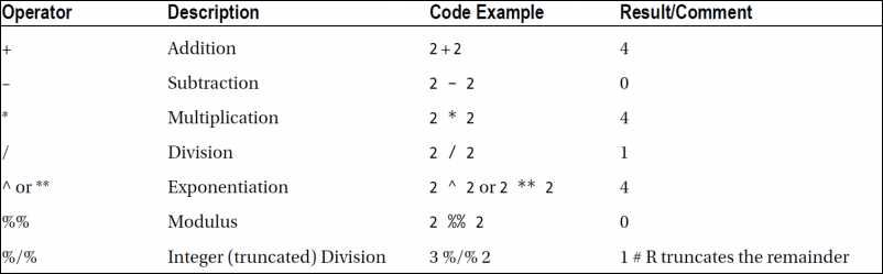
산술 연산자
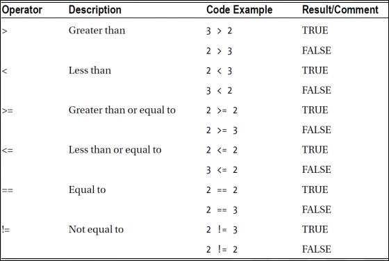
비교 연산자
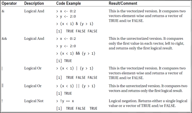
논리 연산자
커스텀 연산자
아래와 같이 연산자를 따로 만둘어 낼 수도 있다.
근의 공식 함수 작성해보기
$ x = \frac {-b \pm \sqrt {b^2 – 4ac} }{2a} $ 을 함수초 작성해보자.
> #Find the real root(s) of a quadratic equation
> quadratic <- function(coeff) {
+ a <- coeff[1]
+ b <- coeff[2]
+ c <- coeff[3]
+ d <- b^2 - 4*a*c
+ cat("The discriminant is: ", d, "\n")
+ if(d < 0) cat("There are no real roots. ", "\n")
+ if(d >= 0) {
+ root1 <- (-b + sqrt(d))/(2*a)
+ root2 <- (-b - sqrt(d))/(2*a)
+ cat("root1: ", root1, "\n")
+ cat("root2: ", root2, "\n")
+ }
+ }

> abc <- scan()
1: 2
2: -1
3: -8
4:
Read 3 items

> abc
[1] 2 -1 -8

> quadratic(abc)
The discriminant is: 65
root1: 2.265564
root2: -1.765564
소수 구해보기
> check_prime <- function() {
+ num = as.integer(readline(prompt="Enter a number: "))
+ flag = 0
+ if(num > 1) {
+ flag = 1
+ for(i in 2:(num-1)) {
+ if ((num %% i) == 0) {
+ flag = 0
+ break
+ }
+ }
+ }
+ if(num == 2) flag = 1
+ if(flag == 1) {
+ print(paste(num,"is a prime number"))
+ } else {
+ print(paste(num,"is not a prime number"))
+ }
+ }

> check_prime()
Enter a number: 3
[1] "3 is a prime number"

> check_prime()
Enter a number: 6
[1] "6 is not a prime number"